Recapping Bayesian Statistics walkthrough from Neuromatch Academy
Fair use
This post is going to walk through tutorials 1-3 on week 2, day 1 of Neuromatch Academy. I’m hoping to add summaries of the tutorials for some of the other days too, eventually. Special thanks to fellow student Maria Khoudary and TA’s Dana Glenn, Kevin O’Neill, and Shawn Rhoads (and the rest of my pod) for walking me through many of these examples.
Bayesian background
It’s worth beginning by revisiting Bayes’ theorem. It turns out that this much talked about theorem is just a specific type of conditional probability. Let’s review conditional probability in a paragraph by referencing this awesome link.
It’s like wanting to know, if I pick a random point, or x value, along that blue bar, what are the odds the red bar also exists at that x value? Essentially we account for this “if” statement with a condition. It means we’re working only within the domain in which that condition is true, and in the case of the bars, essentially zooming our lens to only look at values where the blue bar is.
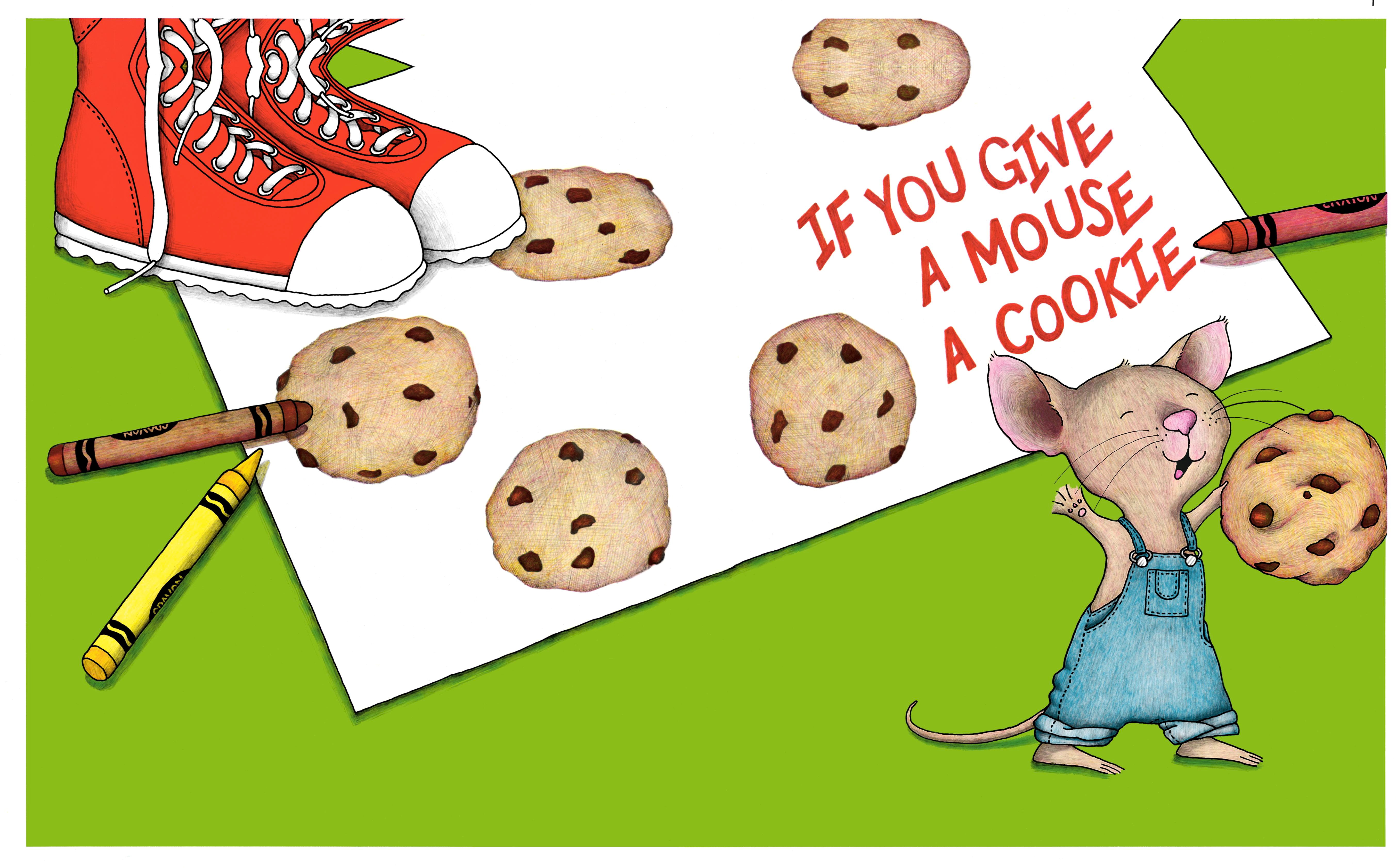
Now let’s make things a little more Bayesian. That example was sort of constant, where the prior, the zoomed in area, was probably the same over time. The beauty of Bayes’ theorem, though, is it allows us to easily update this prior upon new information. Let’s say instead that we want to know the probability that a mouse eats a cookie for dessert (I’m referencing If You Give a Mouse a Cookie). If our mouse thinks highly of cookies, all else equal it’ll probably have a cookie most of the meals it eats. Let’s label this “all else equal” value P(Cookie) = .6, saying that the mouse likes cookies so much it’ll eat one 60% of the time, regardless of the meal. If it had a bad experience with cookies and became less fond of them, or found a new favorite food, the value of this prior would shrink.
If we’re starting from looking at all the mouse eats in a whole day, we also need to zoom in on desserts. So we ask, what’s the probability it’s even eating dessert?. If it eats breakfast, lunch, dinner, and dessert in a day, we’ll coarsely say there’s a 25% chance. In other words, P(Cookie | Breakfast) = P(Cookie | Lunch) = P(Cookie | Dinner) = P(Cookie | Dessert). Suddenly let’s say all else is not equal. Let’s say our mouse is more of a pancake person in the morning, and especially interested in cookies for dessert. If we catch the mouse eating a cookie, then it’s more likely to be dessert than breakfast—P(Dessert | Cookie) should be greater than P(Breakfast | Cookie). We’ll set P(Dessert | Cookie), the likelihood, as .4.
That sets up the conditional probability in this example. We know from the prior how often the mouse eats cookies on average, 60%, and we know from the likelihood that 40% of those meals are just dinner. Therefore, 6 $\cdot$ .4 = 24% of all meals are a dessert in which it eats a cookie. Since we originally wanted to know how likely the mouse is to eat a cookie given that it’s dessert, we can divide .24 by the odds of it being dessert, .25, meaning P(Cookie | Dinner) is 96%, vs (1 - .4 = .6) /3 = 20% across the other three meals.
$$ $$
Ok, so what does that formula have to do with the behavior in the Neuromatch example? Because that behavior is also basically an integration of two pieces of information—instead of taking into account both how much we believe it’s worth eating a cookie and how much our cookie eating comes just from dessert to find P(Cookie given Dessert), we account for both how likely it is that an image appeared in a given location (our prior), and how likely the audio actually comes from where we thought we heard it come from. We’ll get more into this in a moment, but first let’s review the task for tutorial 1 (which note is different than the task for the other tutorials!)
$$ $$
Tutorial 1
So you see an image, you hear a sound, and you have to determine where the sound came from, with the understanding that the image location may have some bearing on where the sound came from. We have that understanding, our prior, because throughout our lives, we’ve come to expect a sound to come from the same place as an object if both just suddenly occur at the same time.
Now we can start plugging into the Bayes equation (or dare I say, equayesian; ok I’ll stop (maybe)). So P(H), our prior, is our existing belief that sudden crossmodal stimulation usually comes from a common source (i.e., if we see a flash of light and hear a crash at the same time, it’s more likely that that sensory information is a product of a single event rather than two independent events). Let’s say we’re positive we saw the visual stimulus at x = 3. And let’s say in general we’re pretty sure that where there’s a visual stimulus there’s sound. In fact, let’s say we’re certain (P(H) = 1). Then P(E | H) won’t influence our selection. We already know where the image was, and we’re assuming that must be where the sound is. And so we respond by saying the sound occurred where the image did. And we keep doing this for a few trials, receiving feedback after each trial.
And then suddenly we’re told our response was incorrect.
In fact, we wind up completing 30 trials and saying the sound is exactly where the image was, and that strategy only leads us to the correct answer, say, 75% of the time. What we’re realizing is that the prior isn’t precise enough to be correct. In other words, there’s uncertainty about the sound location even though we know where the image was. So we adapt.
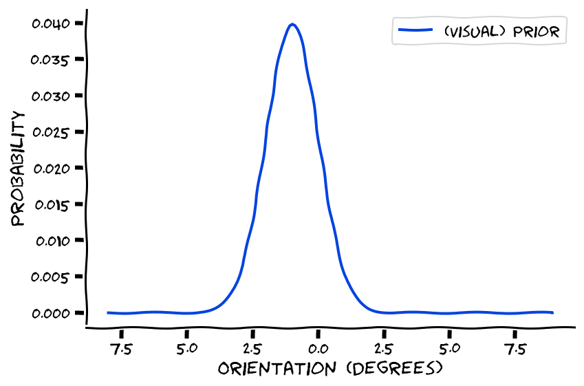
We start changing our strategy, updating our prior to reflect the fact that audio and visual information don’t always come from a common source (P(H) ~= 0.8). Let’s model this (incorporation of) uncertainty. Say the visual stimulus appears at x = -1. We’re now going to create a distribution to represent the likelihood that indeed the sound also occurred at -1. So we create a Gaussian distribution (aka a normal distribution) with the mean indeed at -1, but the standard distribution (representing our uncertainty) spread over a few x values, see below.
Then we also incorporate the additional piece of information, where the brain noisily encodes the sound as coming from. This piece of information also conveys uncertainty, though, since (whereas we’re assuming that if we saw a stimulus somewhere, we’re 100% certain the stimulus in fact occurred there), we’re not so great at localizing sounds (if we were great, perhaps we wouldn’t even need to rely on the prior).
So we’re going to represent our uncertainty about the sound as a Gaussian distribution, too. Say we heard the sound at x = 3, then the mean of the distribution, μ, rests at 3, and we’ll spread the standard deviation over a few values too.
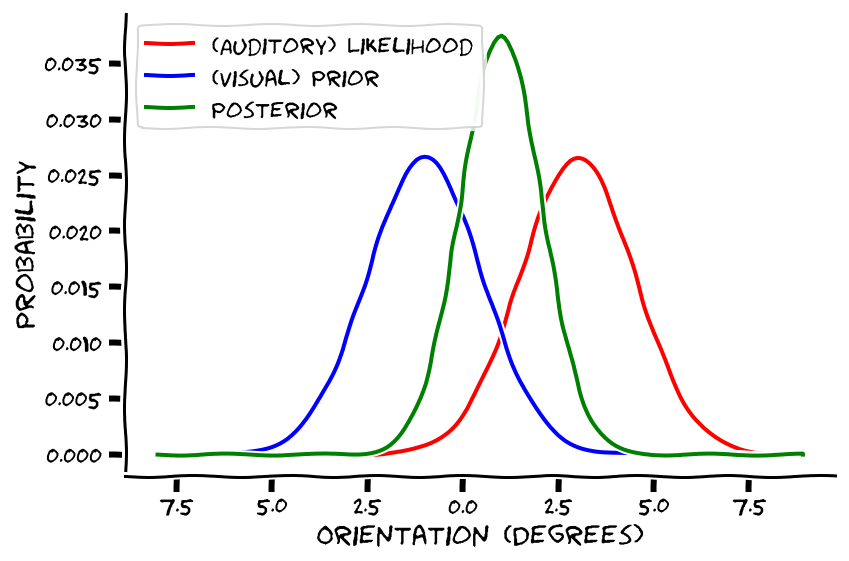
Ok, so now our guess of the sound location is some happy medium between where the image occurred (because that prior is quite meaningful on its own) and how our brain encoded the position of the sound. Then, we do a bunch of trials, and we see and learn about how accurately the image and guessed sound predict the true sound’s location. If it turns out the image location hardly predicts true sound location, there will be a large variance between image location and true sound location, and we’ll choose to emphasize more reliable information, i.e. where we encoded the sound coming from. Conversely, if there’s hardly any relationship between our brain encoding of the sound and where it turns out the sound occurred (learned via trial feedback), we’ll choose to rely more on the image’s position to make our choice. And if both the image location and perceived sound location are unpredictable, well that sucks haha.
This compromise between prior and likelihood gets represented in the following equation. Basically, the Gaussian distributions for image location (the prior) and encoded sound location (the likelihood) combine to form a new Gaussian (the posterior, our guess of sound location), which is a like a weighted sum of the mean and standard deviation for both the prior and likelihood.
$$
$$
Ok, before we move on to tutorial 2, just worth mentioning that I learned the other day that there are MRI scanners for mice! Look at how cute this thing is
Anyways…
Tutorial 2
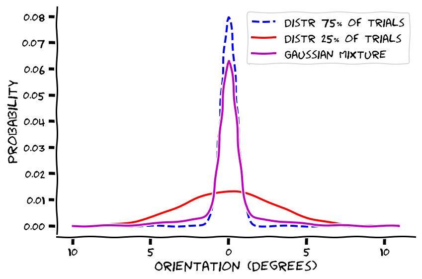
Tutorial 2 is quite similar to tutorial 1! The only thing we’re going to change is one of our assumptions about our priors. Recall we assumed the prior indicated the correct location if one took some variance into account, such that relying only on the prior to estimate the sound location would have yielded about 75% accuracy. In tutorial 2, we keep the prior’s accuracy at 75%, except this 75% takes on a different distribution. Specifically, the prior goes from representing a single distribution to in tutorial 2 representing the combination of two different Gausssian distributions. Tutorial 2 assumes that 75% of the time, our prior is always correct and, because it’s so consistently accurate, should have a negligible variance and standard deviation. In contrast, 25% of the time the image location says almost nothing about the sound’s true location, in which case there is tremendous variability between perceived and true sound location, yielding a massive standard deviation.
Of course, it would be great if we knew at the time whether a given visual stimulus’ location was or wasn’t meaningful. But as a 76ers fan, I know that life’s not fair. So each trial we have to take an amalgamation of the 75% of trials’ and 25% of trial trials’ distributions. They combine to form, you guessed it, another Gaussian, called a “Gaussian Mixture.” This Gaussian Mixture prior then combines with the Gaussian for likelihood to form, you guessed it again, another Gaussian, representing the posterior.
Tutorial 3
Finally, we reach tutorial 3 (there’s also a tutorial 4, but since most groups did not reach it I’m going to skip it here). When I first tried to do tutorial 3 I thought it was the most difficult of the three, but upon understanding it I actually think it’s the most straightforward. I just think some of the wording and graph axes are confusing.
Tutorial 3 sets up an experiment just like tutorial 2, except instead of a 75⁄25 split for the prior it’s 95⁄5, which means the Gaussian Mixture is almost the same as having no distribution whatsoever. The standard deviation is so small for the prior that the prior is going to be extraordinarily influential in the final choice.
Specifically, in 3.2 the prior pretty much assumes that, except for a tiny amount of variance (which is hard to see anyways cause of the dark coloring), the sound location will be at point 0, the location for 95% of trials. Whether it’s going to be influential or not, we can also calculate the Gaussian curve for the likelihood function (3.1; values plotted on the y axis), and sure enough wherever the sound happens to occur at a location other than 0 (5% minority trials) our likelihood model homes in on a similar location, though with some variance like in tutorials 1 in 2, in blue.
That leaves the question of who will “win out” between prior and likelihood. Although I alluded to the prior being particularly influential in this case, the likelihood still holds its own. When the brain encodes a sound as far away from x = 0 (the likelihood, seen on the y-axis), the posterior predicts a location far away from 0, too, but this posterior is quite smeared out by the competing prior. In contrast, near $\tilde{x}$ = 0, the prior and likelihood essentially reinforce each other, with both pointing to the sound coming from around 0. That’s why the posterior is so much brighter in the middle of the graph, the vertical part, than toward the sides.
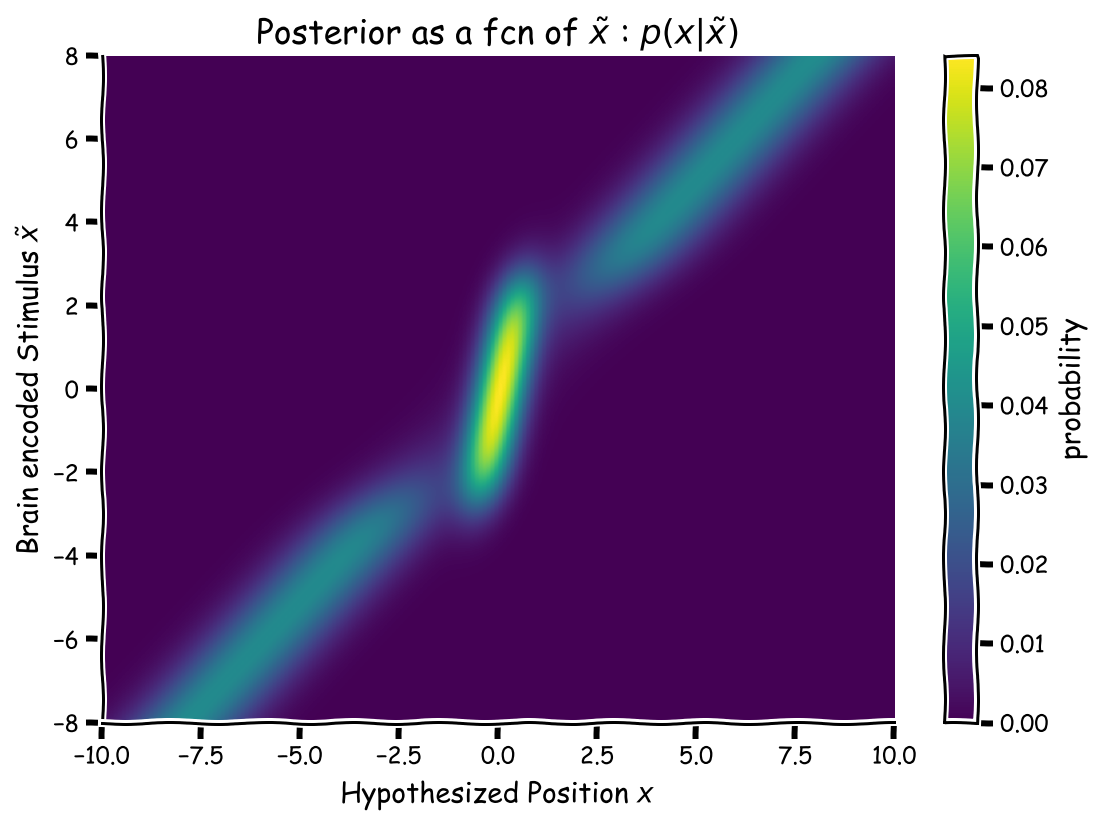
I’d say the novel feature of tutorial 3 is this following part. One of the contributions of Bayesian modeling is that it gives us a normative, or optimal, benchmark of behavior. This is why it’s introduced as a “why” model (see this footnote for an explanation of what, why, and how models1). Performing optimally, a human who’s collected data in the way we’ve described so far and has reached such a posterior should then, of course, respond accordingly. In this case, given the sound actually occurred at some x value, they would respond with the position whose y-axis value is brightest at that x value. They sort of do this in section 3.4, but if the sound had actually occurred at x = 2, then optimal behavior given the posterior would be like stripping down the heat map just to the vertical line x = 2, and then checking which value, in this example ~ 2, was the mean of the posterior’s Gaussian.
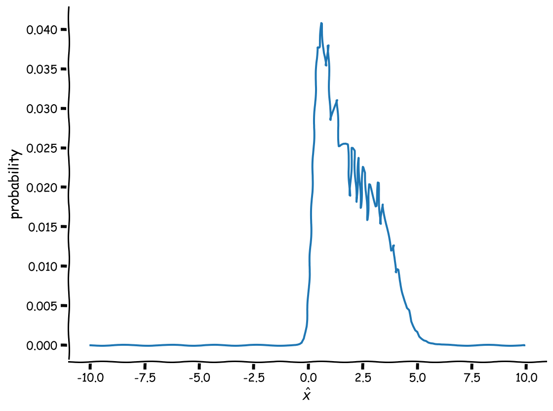
The last part of the tutorial, though, forces us to reconsider whether people behave “optimally” given the posterior they’ve arrived at. In fact, we’re then supposed to assume that we need to multiply the posterior Gaussian (which as a reminder, is a combination of the likelihood Gaussian and the prior Gaussian, which itself is a combination of the 95% and 5% Gaussians) by a Gaussian of how people actually make sense of the posterior. We think sometimes there’s a mismatch between posterior and choice because people, well, make mistakes and lose focus and have limited executive processes, etc (no, definitely not writing a thesis about that, no way, definitely not…).
Probably better Bayesian explainers than what I wrote:
- Chapter from Jonathan Weisberg’s book
- Tim♦’s answer on Stack Exchange
- Dilip Sarwate’s answer on Stack Exchange
- Dana and I walked through a hypothetical that I thought nicely boiled down what vs. how vs. why models. These three models, by the way, are three general frameworks for contextualizing any type of computational model. Fun fact, by the way, I learned only two weeks ago that modeling is just writing a function and then seeing how well that function and its parameters that you’ve chosen characterize the data).
Let’s say we want to study ice cream eating habits. A what question might be, “What do the eating patterns of people look like over the year?” Such a question might lead us to notice that people in the Northern Hemisphere eat more ice cream during July than January (can’t say the cold slows me down, though). The next question might be, “Why do people eat more ice cream during July than January?” to which we might build a model demonstrating that people prefer a cold food like ice cream as a way of cooling down, which is more likely to be necessary during the a warm month like July than a cold month like January. Finally, we might want to know “How,” specifically, “How does the cold ice cream cool you down?” which might prompt a model for how the consumption of ice cream slowly affects maybe your hypothalamus responsible for homeostasis, and that in turn triggers an internal cool down that counteracts all the heat your skin is bringing in (don’t quote me at all on this, I don’t know what I’m talking about). [return]